Jmol/Storymorph
From Proteopedia
This is the documentation for Storymorph, a suite of Jmol functions to help with superimposing and morphing between two structures representing different conformations of a molecule or molecular assembly (script). For more general information, see Jmol/superposition and Morphs. If you load storymorph.spt into a Jmol session where no structures have loaded or all structures have been removed using the "zap" command, it will run a demonstration superposition and morph based on calmodulin strutures. Most examples in this documentation are from this demo.
Overview of capabilities
A superposition of two conformations shows which parts of the structure change the most with respect to the other conformation. For large conformational changes, a morph is easier to understand because it connects the initial and final conformation with a smooth trajectory. This trajectory is like telling a story - it is entirely up to the individual making the morph. For this reason, the Jmol suite is called storymorph. There are three innovative aspects to storymorph.
- Morphs are done on the fly and restore coordinates afterwards, so it becomes possible to try out a lot of different options and explore the two conformations more deeply yet quickly.
- The concept of anchors, ensuring inter-domain connectivity during the morph that does not rely on time-consuming energy minimization.
- The capability of timing the domain transitions independently, giving the viewer a sense of cause and effect. The cause and effect is part of the storytelling, and does not necessarily reflect a true cause and effect.
Try it yourself
If you want to get a feel for the morphs before you read the theory, explore this section. If you don't like pushing buttons without knowing what is happening, skip this section and come back to it later.
| |||||||||||
Worked examples
- To see the changes in the C-terminal domain, move model 2 to minimize distances between the two conformations of this domain (i.e. choose superimpose Cterm). Check the Palindrome box, and display model 1 only. Then, click the morph button labeled "N anchored to C". If you want to focus on the changes in the C-terminal domain, also select the consecutive timing option. Because the C-terminal domain does not undergo rigid body rotation, it is easy to focus on the subtle changes in the conformation.
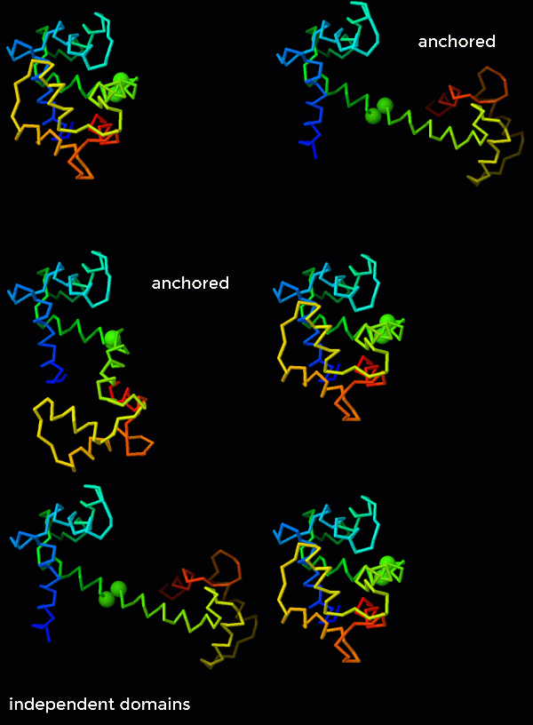
- To focus on the N-terminal domain, superimpose Nterm, and run the "C anchored to N" morph. With this superposition, you can see the (less subtle) changes in the N-terminal domain, while the changes in the C-terminal domain are hardly perceptible. To explore how the anchoring helps to maintain covalent bonds, run the "independent domains" morph instead. To emphasize the distance of the link between the two domains (in this case, the distance between consecutive alpha carbon atoms), choose the "combo" representation and run the two morphs again (see animated GIF on the right.
- To see a bad linear morph, superimpose "Nterm", check "skip rigid" and run any of the morphs. The reason the morph is bad is the large rotation of the C-terminal domain, foreshortening distances (e.g. "flattening" helices) in the middle of the trajectory in the absence of a rigid body movement.
- To see a good linear morph, superimpose "all", check "skip rigid" and run any of the morphs. Because the necessary rotations are smaller in this case, the distortion of the domains is much smaller and hardly noticable as the domains are moving.
Two-phase Morph: rigid body followed by linear interpolation
The morph algorithm is done domain by domain. For each domain, the domains in the two structures are superimposed. and the superimposed domains are gradually moved from the initial to the final orientation. Then, in the second phase, coordinates are interpolated through a linear interpolation. The result is a smooth change in orientation and in conformation. Because there is a rigid body movement in the first phase, positions of a given atom are on curved rather than straight trajectories. To maintain connectivity of covalently linked domains, anchors are used (see below).
Anchors
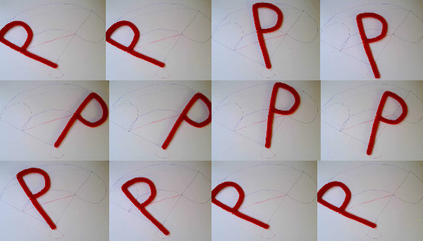
In preparation for a morph, you assign each domain an anchor. If the anchor selection is within the domain, the center of mass of the anchor will move on a linear path from initial to final state. Atoms within the domain but far away from the anchor will move on curved paths if the rigid-body transformation from initial to final state involves a rotation, not just a translation.
In the right example, the midpoint of the "P" travels on a line (faint red line). As a result, the base of the "P", which has the same position in the initial and final state, moves away from this position during the morph. In the left example, the base of the "P" was chosen as anchor. Now it travels on a straight line (or in this case stays put) while the other parts of the "P" travel on curved paths (blue faint lines).
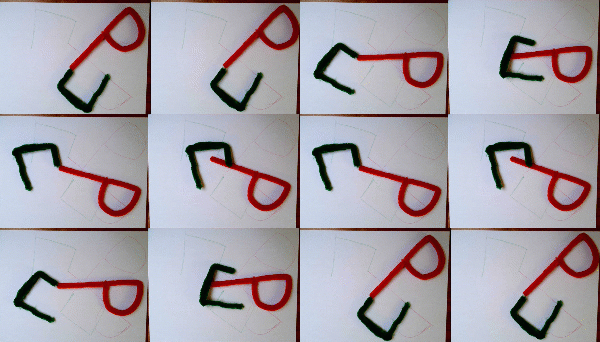
If the anchor selection is part of another domain, the morph algorithm will ensure that the distance of the domain to the anchor remains constant throughout the morph. In essence, the other domain "drags along" the domain in question. To maintain connectivity between domains linked by a single covalent bond, an appropriate anchor would be the atom or residue the domain is directly attached to. If their are multiple covalent connections between domains, you can choose the anchor to include all the connection points.
In the right example, both red and green objects have their respective centers of mass travel on a line. As a consequence, the connection between the objects, which is present in both the initial and final state, opens during the transition. In the left example, the anchor for the green object was chosen to be the base of the red "P". As a consequence, the green object travels on a more complicated path maintaining the connectivity.
Loading the two structures
You can directly load two structures from the PDB into Jmol using the "load files" command, e.g.
load files "=1prw" "=1cll"
model 0
In many cases, a single structure already contains two conformations, such as the two subunits of a dimer, mulitple models in an NMR structure, or multiple copies in the asymmetric unit. You can also assemble multiple structures into a single PDB file, designating them as different models (with the MODEL n and ENDMDL tags).
Defining the two structures
You need to define a variable (called "structures" in the examples) to select the two conformations. Structures is a list of two selections. The selections are enclosed in braces ("curly parentheses"), e.g.
structures = [{1.1}, {2.1}]
Here, the selection is the first and the second structure loaded. For models in a single-structure file, you would use "1.1" and "1.2" instead. For subunits with different conformation, you would select by chain name, e.g. chain="A" and chain="B". More complicated cases are possible (chain B of the second model vs. chain A of the third model) but probably rare.
Defining the domains
Often, conformational changes preserve the fold of entire domains but show differences in inter-domain orientation. Classical examples are the conformation states of hemoglobin or the flexible linker connecting domains of antibodies. For superpositions and morphs, it helps to identify these domains. In storymorph, the domains are collected in a list. Each list contains another list of three selections. The first of these describes the entire domain. The second selection defines the anchor for the morph (explained below). The last one is used for superpositions. Here is an example:
domains = [
 [{78-147},{78-147}, {(78-138)}], // morph 78-147 as unit, use 78-138 for superposition
 [{4-77}, {78}],                  // morph 4-77 as unit, anchored at 78
]
Again, selections are enclosed in braces. If you omit the third selection, or the second and third selection, the first selection will be used (in fact, the functions that require a domain definition will fill in the missing selections).
Implementing the anchors
To ensure connectivity between covalently linked domains, you can set the anchor of the second domain to be the connecting residue of the first. For example (see domain definitions above), the first domain might be {78-147} and the second domain {4-77}. To make sure the second domain does not get detached, we would choose the anchor as {78}, within the first domain and directly connected to the second. Because of the anchors, the order of domain definitions becomes important. Anchors either have to be within "your own" domain (for a linear movement of the anchor), or in the domains higher up in the list. The latter ensures that we already know where the anchor is before we translate the current domain to maintain the appropriate distance to it.
Loading the storymorph suite
If you have internet access, this command will load the script. With an open console, it will also give some basic reminders of the functionality:
script "https://proteopedia.org/wiki/images/a/a2/Storymorph.spt"
If you are working in Proteopedia, you should shorten the link to make it local:
script "images/a/a2/Storymorph.spt"
Superposition
The superimpose function works the same way as the Jmol compare function, but it first verifies the required atom selections to prevent Jmol from crashing or freezing. The superimpose function takes two or three parameters. The first paramenter always defines the two structures (see above). The second parameter is either a single domain selection (when calling with two parameters), or it is the list of list describing all domains, with the third parameter an integer designating which domain is to be used in the superposition. The superposition leaves the first structure in its original orientation and moves the second structure to minimize the distances between corresponding atoms (defined by the domain selection). Different from the morph function, the superposition function alters coordinates for the remainder of the session. Because morphs connect initial and final atomic positions with a path, the orientation of the final state with respect to the initial one is crucial, and the choice of superposition defines this orientation. In other words, you get a different morph if you choose to superimpose the two structures in a different way before starting the morph.
To superimpose the two structures by minimizing distances in a given domain, use the superimpose() function. For example,
superimpose(structures, domains, 1)
would superimpose the two structures based on minimizing distances in domain 1. You can also run the function with two paraments. In this case, the second parameter is a selection of the atoms you want to superimpose. To superimpose all carbon alpha atoms, you would run:
superimpose(structures, {alpha})
Notice the braces surrounding "alpha" to designate an atom selection (or atom set in Jmol terms). This only works if the number of selected atoms is the same in either structure. It will only give a meaningful result if the atoms in either structure are ordered such that you get matching pairs within the selections.
Running the morph
Once you superimposed structures and defined domains, you are ready to start the morph. In our example, the command is:
morph(5, structures, domains)
This generates 4 intermediates (5 steps of the morph, or a total of 6 structures including initial and final given structures). The morph command saves coordinates first, then alters coordinates during the morph and restores them afterwards. This way, you can run morphs consecutively without having to reload coordinates.
Timing
Storymorph allows you to control the timing of transitioning from initial to final conformation at a domain level. So you could first have one domain undergo conformational change and then the second, or have everything happen at the same time. The timing information is collected in a list with the same number of items as there are domains. Each item is a list of three numbers. The first two say when the transition from initial to final state should happen (0 and 1 mean throughout the morph, 0.2 and 0.5 e.g. would mean start 20% into the morph and complete 50% into the morph). The last number, when different than zero, means that the domain will be rotated in the "long" direction (e.g. if it takes a 30-degree rotation in one direction to superimpose initial and final orientation of the domain, a 330-degree rotation in the other direction is applied).
For a 2-domain morph, with default timing, you would set:
timing = [
[0, 1, 0],
[0, 1, 0],
]
If you want to show the changes in domain 1 and 2 consecutively instead of simultaneously, you would instead set:
timing = [
[0, 0.5, 0],
[0.5, 1, 0],
]
To run a morph with this timing, the call is the following:
morph(10, structures, domains, timing)
If you leave out the fourth parameter, the timing will be set to the default (all at once).
Parameters
You can modify the behavior of the morph() function by setting certain parameters before you run it.
- morph_delay = 0.5 for 0.5 seconds dalay between frames
- morph_savefiles = 1 for saving frames to file
- morph_pause = 6 for pausing at frame 6
- morph_palindrome = 1 for returning back to the start
- morph_skiplinear = 1 for skipping the linear morph when debugging
- morph_skiprigid = 1 for skipping the rigid body move when debugging
Helper functions
When making a new morph, a lot of time is spent on figuring out the matching atoms between two structures (there might be missing residues, incomplete sidechains, altloc multiple conformations, mutations, inconsistency in residue numbering, unconventional order of atoms in the file, some residues labeled as HETATM instead of ATOM etc.).
There are two helper functions to speed up the process of finding matching atoms.
The function matched_residues() walks through the two structures residue by residue, checking whether there are the same number of atoms. The function has two parameters, sel1 and sel2, representing the two selections. You can specify the selections directly, as in:
matched_residues({:A},{:B})
which would check which residues in chain A and chain B match. In the output, "all" means that there are the same number of atoms, and "some" means that the residue number exists in both selections, but has a different number of atoms. To explore why, you can limit the selection to mainchain or alpha, or exclude alternate conformations ("not *.%B") and run matched_residues with the limited selections.
If you already set up the "structures" and the "domains" variables, you can test a given domain (say domain 2) by running:
matched_residues(structures, domains, 2)
Once you have verified that you have the same number of atoms in two selections, you can also verify that matching atoms occur in the same order using the atom_order() function:
atom_order(sel1, sel2)
or
atom_order(structures, domains, 2)
where the last parameter gives the domain to compare (in this case domain 2).
Examples complete with code
Calmodulin
load files "=1prw" "=1cll"
delete water
delete protein and not alpha
model 0
backbone only
backbone 0.2
display 4-147
color group
structures = [{1.1}, {2.1}]
domains = [
  [{78-147},{78-147}, {(78-138)}], // morph 78-147 as unit, use 78-138 for superposition
  [{4-77}, {78}],                  // morph 4-77 as unit, anchored at 78
]
script "https://proteopedia.org/wiki/images/a/a2/Storymorph.spt"
superimpose(structures, domains, 1)
center visible
model 1
morph(5,structures, domains)
Hexokinase
load "https://proteopedia.org/wiki/images/f/f2/Apo_hexokinase.pdb"
load append "=3O8M"
select all; cartoon only

structures = [{1.1 and not *%B and not *%C},{2.1 and not *%B and not *%C}]
domain2 = {82-210}

domains = [
[{protein and (14-486) and not domain2},
 {protein and (17-486) and not domain2},
 {protein and (17-486) and not domain2}],
[domain2, {(81,211)}]
[{glc}],
]

timing = [[0, 1.0, 0],[0.3, 1.0, 0], [0, 0.41, 0]]

select glc
spacefill on
select protein
color tan
backbone only
backbone 0.2
select within(3.5, glc)
select within(group, selected)
select selected and (sidechain or alpha)
wireframe 0.3
select selected and sidechain
color cpk

script "https://proteopedia.org/wiki/images/a/a2/Storymorph.spt"
morph(20, structures, domains, timing)
Storymorphs on Proteopedia
The following pages contain morphs created with the Jmol script:
Recoverin, a calcium-activated myristoyl switch
SARS-CoV-2 spike protein fusion transformation
If you use Storymorph to make your own morphs, please add the following to your references:
<ref>The [[Jmol/Storymorph|Storymorph Jmol scripts]]
were used to create the interpolation shown in the morph.
[https://proteopedia.org/wiki/index.php/Image:Spike_SARS_CoV_2_storymorph.pdb|Coordinates]
available on Proteopedia</ref>
If the morph is made on the fly in Proteopedia, please reference as:
<ref>The [[Jmol/Storymorph|Storymorph Jmol scripts]]
creates the interpolated coordinates
of the morph on the fly.</ref>
This way, there will be an easy way to find all Storymorphs on the site, and readers can learn about the method used.


